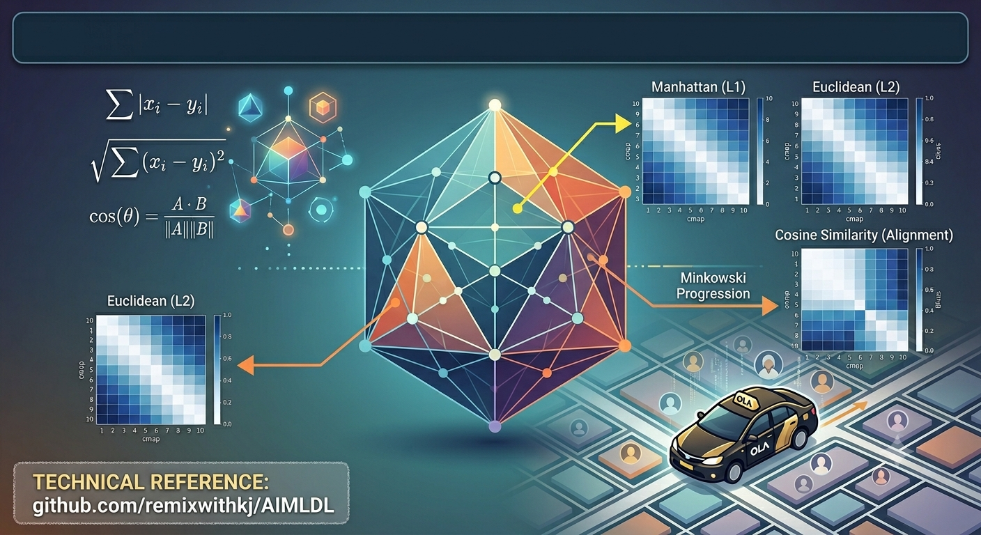
Marketers and business leaders frequently navigate complex segmentation challenges—from optimizing promotional campaigns and product distribution to refining SKU variants—by organizing diverse ‘things’ into logical, actionable cohorts.
Those ‘things’ could be customers, products, transactions, employees, documents, locations, user behaviours.
To create these logical clusters, one must be able to predict with certainty exactly how similar or different two entities are. We are constantly faced with questions like:
- Which customers are similar, and to which segment do they belong?
- What products must be recommended to similar customer sets?
- Is a particular transaction a regular, high-value event, or a dangerous outlier?
The notion of distance and similarity is the building block powering the fundamental architecture of modern Machine Learning. These metrics act as the precision tools required to transform raw, disparate data into confident, actionable business insights.
What is notion of distance or similarity in machine learning?
Distance and similarity are fundamental building blocks of all machine learning techniques and algorithm.
Think of them as indefatigable soldiers who power ML algorithms and are backbone of several strutuctured problem solving
Let us look at some ML algorithms and the distance metrics which support them.
| Type of problem/Algorithm | Distance or Similarity measure |
| Unsupervised Clustering or Classification e.g. K Means, KDE or Parzen window, Agglomerative clustering | K Means clustering: Standard implementations use Euclidean distance, this default metric structure can be tuned depending on the dataset features. KDE or Parzen Window (Kernel Density Estimation): Defining how the distance between data points is calculated changes on how the density functions evaluate proximity. Standard scikit library allow switching the underlying metric hyperparameter alongside the bandwidth parameter. Agglomerative Clustering: Explicitly requires a distance metric hyperparameter to build its proximity matrix, coupled with a linkage criterion (to be discussed later) |
| Supervised classification e.g. KNN, SVM, Mixture of Gaussians etc. | K-NN (K-Nearest Neighbors): The choice of how proximity is computed (e.g., Euclidean vs. Manhattan distance) is a core hyperparameter. SVM (Support Vector Machine): Uses a kernel function hyperparameter (like RBF, Polynomial, or Linear). The RBF kernel uses squared Euclidean distance. Mixture of Gaussians: Relies on a statistical distance (Mahalanobis distance) natively derived from covariance matrices, rather than a user-chosen distance metric hyperparameter. Mahalanobis distance is the most nuanced distance metric and shall be discussed at length |
| Collaborative filtering and recommender system | All user-similarity based and object-similarity based recommender systems used distance metric as measure of proximity |
| Optimization Problems | All optimization problems either direct in nature or disguised as as ML algorithm use distance metric. e.g. K-Means at heart is an optimization problem. Think of it like an optimization problem where the objective function is minimising intra-cluster variance and maximising inter-cluster variance or distance. |
What is a ‘metric’ anyway?
The word “metric” has a rich, deep etymology.
The word metric traces back to the Ancient Greek metron, meaning ‘a measure’ or ‘that by which anything is measured.’ While it was originally used to describe the rhythm of poetry or the physical length of objects, it has slowly evolved to define the ‘geometry’ in the current context.
To be called a metric or measurement, the 3 axioms of Identity, Symmetry, Triangle Inequality must hold true.
1. Identity of Indiscernibles (distance to self):
The distance from a point to itself must be exactly zero: distance(x, x) = 0. That is to say, if the distance between two points is zero, they must be the same point.
2. Identity of symmetry:
The distance from x to y must be the same as the distance from y to x: d(x, y) = d(y, x). Whether you are measuring the travel time from your home to the office, or the office to your home, the geometry remains the same.
3. Identity of Triangle Inequality:
d(x, z) <= d(x, y) + d(y, z). In simple terms, a “direct path” between two points will always be shorter than (or equal to) taking a detour through a third point (y).
Fun fact: Some common similarity measures (like certain types of correlation-based similarity) violate the Triangle Inequality.
Cosine Distance is not technically a formal distance metric because it violates the triangle inequality—yet, it remains the backbone of text-based machine learning. More on this later!
Foundational – “Similarity vs. Distance”
- Distance measures “separation” and typically exists on a scale from 0 to inifinity. Crucially, only formal distances adhere to the Metric Axioms.(Identity, Symmetry, and Triangle Inequality) that we discussed.
- Similarity measures “affinity” and typically exists on a scale from 0 to 1.
Here is a simple and elgeant transformation between distance and similarity.
conversely
This relationship ensures that as distance approaches zero (perfect identity), similarity approaches one (perfect match).
Intuitively, this is logical and also stands to vet axiom 1 i.e. Identity of discernibles(or distance to self).
What are the most commonly used distance metrics?
Distance metrics can be split in 7 logical blocks.

Some of the distance metrics metioned above are nuanced and carry wider application, much beyond the taxonomical classification that has been made above.
For example, Jaccard can be used for continuous variables as well. That variant is called the Jaccard generalised distance.
Mahalanobis distance sharpens the Euclidean distance by first normalising the distance (Scale invariance) and then does correlation blending (covariance matrix to collapse correlated dimensions).
How does one eat an elephant?
“One bite at a time.”
Distance metrics—the topic is fundamental, exciting, and expansive. Because of its scale, I will be breaking it down into three digestible, “byte-sized” chunks.
For this inaugural part, we will master metrics dealing with continuous variables (excluding Mahalanobis) and angular variables.
Part 2 will be a deep-dive into shape-aware metrics: Mahalanobis distance (believe me, it deserves a dedicated chapter!), KL divergence and Bhattacharyya distance.
The final installment, Part 3, will cover categorical vectors, sequences and geospatial variables.
What about the implementation?
- We shall first discuss metrics alog with context and applications.
- Metrics are seldom used in isolation, but their thorough understanding is essential to enable algorithms for accuracy and explainability.
- We shall then write code blocks in Python using scikit APIs and Ola dataset.
Continuous Variable metrics – the most commonly used distance metrics?
Distance Metric: Euclidean
Context: The earliest and most commonly used metric.
The coordinate Geometry and cartesian coordinate system in 2D and 3D are more specific applications of this metric.
Technically, it measures the straight-line distance between two points in a Euclidean space (L2 norm)
Applications: Ideal for problems involving continuous real numbers e.g. age, income, sugar level, customer rating etc.
Challenges: Does not behave well with encoded data e.g. when ordinal or nominal data is encoded to 0, 1, 2 etc.
Also loses sense of distance when scales vary too much. e.g. age and income distance between 2 individuals. Person X making 500K at the age of 42 versus Person Y making 1M at the age of 45. With 3 units variation in age, the variation in income is 500K.
A good practice is to scale data points before getting into deeper analytics. (Scaling to be covered later)
Suffers from the ‘Curse of dimensionality’ In high-dimensional spaces, the Euclidean distance between any two points converges and becomes nearly equal. Because every point becomes roughly equidistant from every other point, the metric loses its ability to effectively distinguish between “close” and “far” neighbors.
High Sensitivity to Outliers – Because the Euclidean formula squares the differences across each dimension, it places a disproportionately heavy penalty on large differences.
Representation/resources:

Distance Metric: Manhattan
Context: Measures the distance traversing only axis-parallel segments.
Technically one has to move along axes to the end points to calculate the Manhattan distance
(L1 norm)
Applications: While Euclidean distance assumes a flat straight line distance between 2 points, Manhattan takes a more pratical view and assumes grids as they would be in city streets.
It only allows for grid constrained movement along axes.
Challenges: The grid movement can become a constraint in scenarios where ‘as the crow flies’ would apply. e.g. It would be impractical to use Manhattan while finding distance between 2 points for a flight path, Euclidean or Haversine would be more suited.
Representation/resources:

Distance Metric: Minkowski
Context: It’s really a framework for definition of distances and Euclidean & Manhattan are specific cases.
Applications:

if P = 1 in the above formula then it represents a very specific case of Manhattan distance (L1) while at P = 2, it represents Euclidean distance (L2)
Urban healthcare distribution has successfully utilized Minkowski distance to model realistic travel times across compound infrastructure road networks. For instance, a tuned value of P = 1.31 was mathematically shown to be the optimal measure for evaluating geographic access to emergency cardiac services.
Access research paper at https://doi.org/10.1186/1472-6963-9-200
Challenges: Minkowski has all the drawbacks of the Euclidean as well as Manhattan distances with the added complexity of tuning the parameter ‘P’.
Representation/resources:

Distance Metric: Chebyshev
Distance Metric: Chebyshev
Context: Chebyshev is another special case of Minkowiski distance where P -> ∞.
It is also called the L ∞ norm.
it is interesting to tranform general Minkowski equation
to Chebyshev distance i.e.
D(X,Y) = maxi(|xi – yi|)
Applications: It is often called the “Chessboard distance” because it reflects the exact number of moves a King needs to travel from one square to another. Say the king needs to move from X to Y
where X = (3,2)
and Y = (1,6)
Then D(X,Y) = max(|3-1|,|2-6|)
= max(2,4) = 4.
it is used in applications like Robotics & Automated Warehouse Gantries where independent motors control the horizontal ($x$) and vertical ($y$) axes concurrently at the same speed, the total time required to position a tool or crane is entirely dictated by whichever axis has to travel the furthest.
and Computer vision where the model utilizes “8-connectivity”—meaning a central pixel is considered touching all 8 surrounding neighbors (including those sharing only a corner diagonally)—it relies on Chebyshev distance to determine a uniform 1-pixel radius of connection.
Challenges: Chebyshev has most drawbacks of the Minkowski distance family and some more.
Faithful to one and blindness to all Other Dimensions: The most significant flaw is that it completely ignores variations across all other features except the single maximum difference which means that it loses significant cumulative distance information.
Scale sensitive and hence extremely Sensitive to outliers – Would require normalization in most cases.
Representation/resources:

Distance Metric: Canberra
Context: Canberra distance is a significant enhancement over Minkowski family of distances. It can be thought of as a weighted version of the Manhattan distance that functions by summing up the absolute differences between two vectors divided by the sum of their absolute values across each dimension.

Applications: Say we have 2 vectors.
A (1,0,3)
B (2,0,1)
1. |1-2|/(1+2)= 1/3= 0.33
2. |0-0|/(0+0) = 0 (considered 0 )
3. |3-1|/(3+1)=1/2 = 0.5
Total distance = 0.33+0+0.5= 0.83
One of Canberra’s specific application is Fraud detection where it can generate large suspicion score on specific penny-amounts, low-frequency transaction types, or obscure fees.
Challenges: Canberra holds advantages over the Minkowski as it doesn’t require any normalisation and binds values [0,1]. It is extremely resilient to outliers.
Canberra is also useful in sparse matrix calculations since it completely drops out 0s from the calculations.
Canberra scale has extreme Sensitivity to Small Fluctuations Near Zero and insensitivity to large numbers.
e.g. distance between 0.01 and 0.05 is 0.67.
while the distance between 100,000 and 101,000 is 0.005.
Angular/vector variable metrics – ‘soul saver’ for sparse matrix.
Distance Metric: Cosine distance
Context: Cosine distance considers the additional feature of direction or orientation. This is against just the distance being measured by Euclidean or Manhattan.
Simply put, if we have 2 vectors A & B. Then Cosine distance = 1 – Cosine similarity (A,B).
Cosine similarity (A,B) = Dot product (A, B)/(||A|| ||B||)
Cosine similarity varies between 1 (for similar or almost identical) to -1 (diametrically different). Hence Cosine distance shall vary between 0 and 2.
Applications: Text mining and NLP: Article A is 500 words long. Article B covers the exact same topic but is a comprehensive 5,000-word analysis. Cosine similarity evaluates the proportional distribution of the vocabulary. Because the word vectors point in the same directional cluster, it correctly identifies them as highly similar. While Euclidean distance would have placed these far apart based on the length singularly.
Collaborative filtering in recommender system: User 1 is a film critic who has rated 1,000 movies on a scale. User 2 is a casual viewer who has rated only 5 movies. If their proportional taste profile leans toward the same genres (e.g., sci-fi and indie drama), their directional vectors align. Cosine similarity recognizes this shared taste preference, bypassing the massive volume discrepancy in their streaming histories.
Excels in most embedding based neural tasks where context and sequence of the words are important.
Challenges: Blind to scale: Consider two e-commerce shoppers. Shopper A buys 1 laptop and 1 phone charging cable. Shopper B buys 50 laptops and 50 phone charging cables for a corporate office. Cosine similarity views their purchase vectors as identical.
Misleading Metrics on Highly Sparse Data: If two users have long sparse vectors but share just one minor item in common. Cosine similarity can output an artificially high score based on a single coincidental intersection.
Poor Performance with Negative Values: When vectors contain a mix of large positive and negative numbers, the directional intuition breaks down.
Mean centering must be done else Cosine will output flawed score. e.g. User A rates movis X & Y as [5,5] while User B rates them [1,1]. Cosine similarity will be 1 for them which is flawed. However once the data is mean centered i.e. [5-3,5-3] = [2,2] and [1-3,1-3] = [-2,-2], the similarity is 0.
Representation/resources:

Code level implementation and takeaways.
Generating insights from raw data.
- Step 1: Establishing the Sandbox – I started by selecting the OLA Trip Dataset, a perfect high-dimensional playground. Because ride-hailing data naturally contains everything from rider age and income to complex trip coordinates, it allowed me to test a vast “toolkit” of distance metrics rather than just relying on simple math. The dataset had ~49,000 unique customer data, however to manage compute power, distances were calculated for 100 customers only.
- Step 2: The data had to be imputed and normalised (exciting topics both of these, but for some other day) before getting into pairwise distance calcuations. The link to the codebook and the output is embedded at the end. The dataset had following features (columns) and types.

- Step 3: Protecting the Identity (Index Isolation) – Raw data tables are cluttered with text. I moved the
Customer IDfrom a standard column into the DataFrame Index. This was a vital engineering “shield”—it kept our ID labels safe while ensuring our numerical feature matrix remained perfectly pure for calculation, preventing type-mismatch errors. - Step 4: Algorithmic Sanity (Downsampling) – Distance calculations grow quadratically (N^2). To prevent my notebook from freezing, I performed a deterministic downsample of 100 records only using a fixed
random_state. This would help with reproducibility. - Step 5: The Geometry Portfolio – By computing everything from Manhattan and Euclidean to the more advanced Chebyshev, Minkowski, and Canberra metrics and finally Cosine (distance/similarity) I transformed abstract numerical vectors into a multidimensional proximity report.
- Step 6: Bridging Geometry & Identity – I mapped these raw results back to the original
Customer IDs by wrapping the output matrices into labeled Pandas DataFrames. This restored context, allowing me to compare various distance matrices for reader’s conviction.
I shall now present Pairwise distance metric for various metrics. For readers’ ease distance matrices have been illustrated for 5 customers only. Larger distance matrix (upto 100 X 100 customers)can be referenced from the appended code book.

Euclidean(L2 norm) and Minkowski(p=2) produce identical results.

and Manhattan (L1 norm) and Minkowski(p=2) produce identical results too!

One can also see that and Chebyshev (L-inf norm) and Minkowski(p=inf) are identical.

Observe the progression of Minkowski metric.
p values between 1 and 2 are generally used for more practical scenarios where Manhattan(p=1) and Euclidean(p=2) are too idealistic/unrealistic. Such a study has been referred to where actual distance time-calculation has been done at p = 1.3 for medical emergencies.
Chebyshev (L_infinity norm or p = infinity) focuses on the single greatest difference rather than the sum of all differences.

Comparative for Cosine metric along with Euclidean matrix. Cosine similarity and distance are complimentary hence they will always sum to 1.
Despite different applications, it can be observed that both Euclidean and Cosine metrics deliver similar (not identical) results.
E.g. distance between customer IDs 691197 (last row) and 379207 (first column) is lowest per Cosine metric and second lowest per Euclidean metric.
The annotated codebook can be downloaded from the hyperlink.
https://github.com/remixwithkj/AIMLDL/tree/main/distance-similarity-metrics
That’s all for Part 1. Read Part 2: here
Leave a Reply