Why 30 Data Points? The Golden Rule, Checked

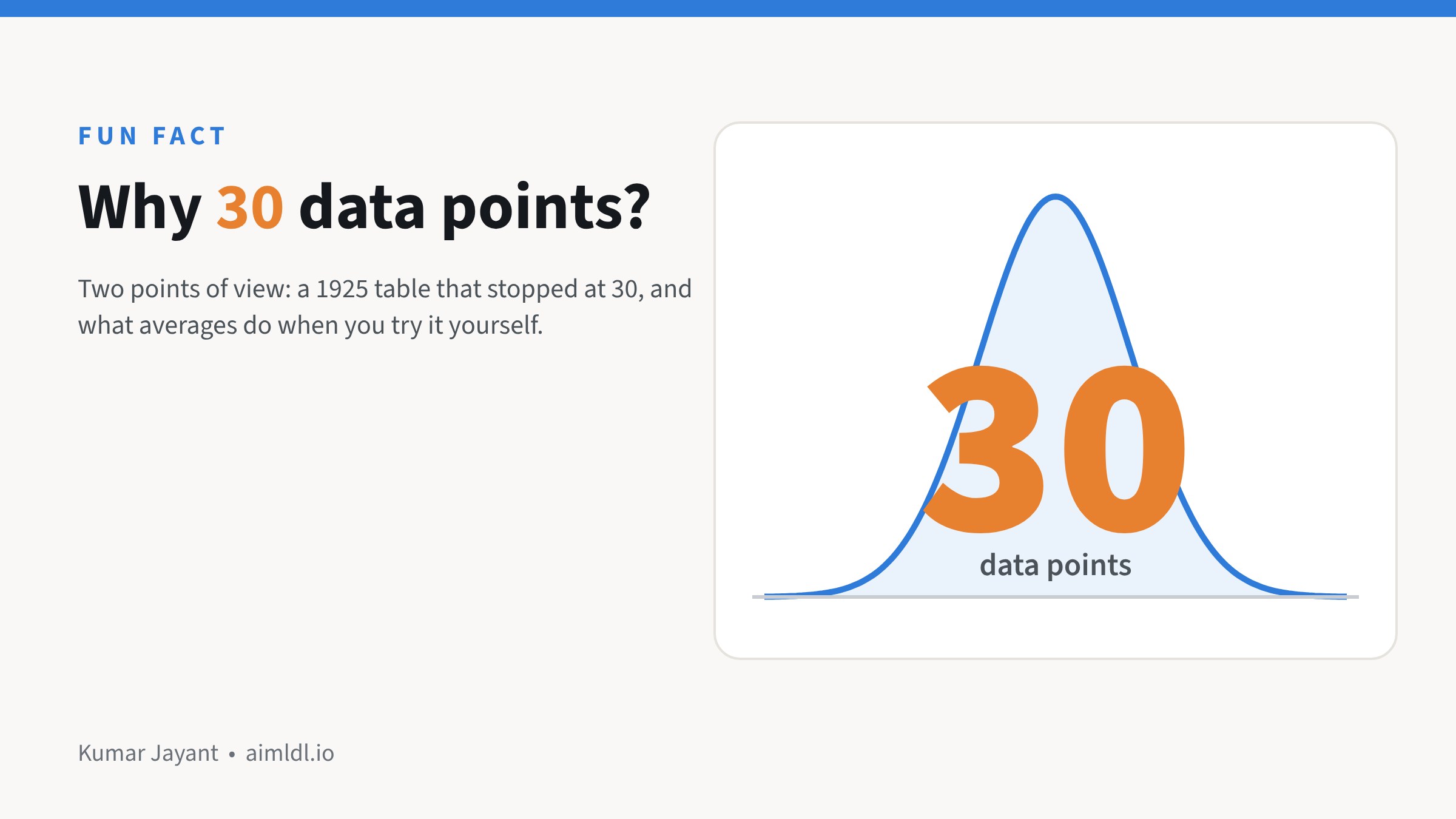
Golden rule of 30 data points: an observation coming from 30 data points is significant, statistically so.

I followed the trail and came across two points of view.

Point of view 1, historical fact:

1925: Ronald Fisher printed the cut-offs in a table that ran from 1 to 30, then jumped straight to infinity. He did all the calculations by hand, pretty intensive stuff. Between 30 and infinity, the two answers barely differ. “Close enough” hardened into a rule.

Point of view 2, observational:

Take 500 data points, say the minutes a quick-commerce service takes to deliver to your home. Draw 2 random points from this set, calculate the average and plot it. Repeat this 1,000 times. Then repeat the experiment with 10 random points, and then with 30.

At 30, a nice bell appears. Beyond 30, the bell takes a sharper shape, and with larger samples it becomes indistinguishable from a normal curve.

Why does it seem to work? Averages behave better than data. Average 30 delivery times, again and again, and those averages form a neat bell curve.

Try it yourself

You can run point of view 2 in five minutes in Excel or Google Sheets.

Excel 365:

=AVERAGE(TAKE(SORTBY($A$1:$A$500,RANDARRAY(500)),2))

Google Sheets:

=AVERAGE(ARRAY_CONSTRAIN(SORT($A$1:$A$500,RANDARRAY(500,1),TRUE),2,1))

When I ran it, the 500 delivery times were lopsided (skew 1.8). Averages of 2 were still lopsided (1.1), averages of 10 were getting there (0.5), and averages of 30 were close to a bell (0.2).

One rule makes or breaks the experiment: keep 1,000 averages every time and change only how many numbers go into each one. Plot just 10 averages and any histogram looks lumpy, however many numbers sit behind each.

Where the “30 rule” quietly runs your business

• A new display is piloted in 30 stores, and the average uplift decides the national rollout.
• Thirty dealers are surveyed, and the average score becomes “what the market thinks”.
• A sales manager is judged on 30 visits, or a new scheme on its first 30 orders.

Each of these feels like enough. Whether it is depends on the numbers behind it.

When 30 is fine, and when it isn’t

• Fine: steady, evenly spread numbers such as delivery times, call durations or ticket resolution times. The average of 30 is a fair guide.
• Not fine: lopsided numbers such as order values, dealer sales or project sizes. One big order can make a pilot look like a winner, or hide a loser.
• Not fine: rare events. If 2% of visitors buy, 30 visitors usually give you zero or one sale. You can’t read a conversion rate from that.
• Not fine: when you slice it. Thirty stores split across five regions is six per region, and six is a story, not evidence.

What to ask yourself or your team before you trust an average

1. Show me the spread, not just the average. A simple chart of all the values is enough.
2. Take out the one or two biggest numbers. Does the conclusion still hold?
3. How many are in each slice we’re comparing: region, channel, customer type?
4. Give me a range, not a single number: “uplift between 3% and 9%” is a decision you can make; “6%” alone isn’t.

For the analyst in you and your team

Plot the histogram before you compute the mean. If it’s heavily skewed, look at the median or the log of the values, and bootstrap the mean to see how much it moves from sample to sample. For tests and pilots, size the sample from the effect you need to detect, not from habit. Thirty is a starting point for a quick look, not a sample-size calculation.

What’s an inherited “rule of thumb” in your business that you’ve never checked?

Sources: W. S. Gosset (“Student”), “The Probable Error of a Mean”, Biometrika, 1908. R. A. Fisher, Statistical Methods for Research Workers, 1925 (table of t). Charts are simulations.

For a full step-by-step analysis, see All Customers Are Equal, But Some Are More Equal Than Others: RFM, Step by Step.